Scripting figures in MRIcroGL

Here I’ll briefly break down (some of) the scripting options for creating figures in MRIcroGL. Like MRIcron, Chris Rorden’s MRIcroGL is a really powerful and flexible tool for visualizing MRI images and statistical results.

Benefits of scripting your figures

In addition to using MRIcroGL to just open and scroll through NIFTI files, I find it super useful for creating manuscript figures. You have a ton of different options that can be tweaked, in addition to nice rendering. Most importantly, you have a python-based coding option so that you can create reproducible figures so you can easily tweak your figures later, adapt figures for future papers, etc.

MRIcroGL possibilities

First, you’ll want to open the scripting panel. To start your own script for a figure, go to Scripting > New. In the scripting menu, you’ll also see multiple templates. Click through the different templates to get a sense of what’s possible in MRIcroGL (a lot!). Before I forget, here is the link to Chris Rorden’s wiki page that provides a ton more detail on MRIcroGL scripting. I will go through just one beginner example here, but his site has a lot more detail. This link to one of the MRIcroGL GitHub pages is also helpful for providing scripting examples.

Using MRIcroGL to create a fMRI results image

Now, back to our goal — to make a fMRI results figure. In my case, I want to make a “mosaic” image that shows different brain slices, with fMRI activation overlaid. I also want a 3D rendered brain to show from which portions of the brain I obtained these slices. So, as I said before, start with Scripting > New (or you could select the mosaic template script as a starting point).

First, a few basic things. You can write / edit your scripts directly in the Scripting panel in MRIcroGL; e.g., you could copy-paste what I have below, edit it, and run it all in MRIcroGL. Use CTRL+R to run scripts in MRIcroGL. Alternatively, you can write in your favorite text editor (e.g., Notepad++), save as a *.py file, and then open it in MRIcroGL (Scripting > Open). Note that if you do this, MRIcroGL will automatically execute the script after opening it… so don’t open it in MRIcroGL unless you want this to happen! (E.g., don’t open it if it includes a save command and you don’t want to save over your previously-created image!) Regardless of where you work on a MRIcroGL script, you’ll definitely want to save your script for later use — to adapt for making new figures or to go back and tweak your original figure. Finally, note that in the bottom righthand corner, you’ll be able to see if your script successfully executed or not. If it worked, you’ll see a happy message. If not you’ll see errors. Happy message:

Running Python script
Python Successfully Executed

Load your images

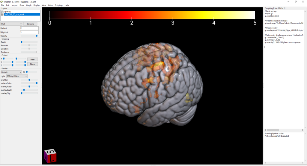
Now for the scripting and figure creation. In this example, I’m going to use the MRIcroGL spm152 template as my underlay. This is found in the MRIcroGL install folder. I’m then going to add my fMRI results image as an overlay. I obtained this results image from saving my statistically thresholded (in this case at FWE<0.05) results image from the SPM results GUI. Also- make sure your slashes are / not \, it matters here.

# Basic set-up 
import gl
gl.resetdefaults()

# Open background image
gl.loadimage('C:/Users/admin/Documents/MRIcroGL_windows/MRIcroGL/Resources/standard/spm152.nii')

# Open overlay
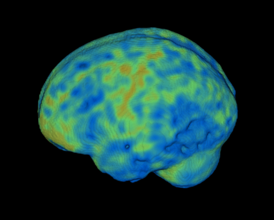
gl.overlayload('E:/VEMP/Scripts/WB_second_level/02_longitudinal_SwE/set1_BG_masked/SwE_FWE_05_pos_mask.nii')

Hit CTRL+R to run. This gives us a pretty basic rendered brain with the overlay added.

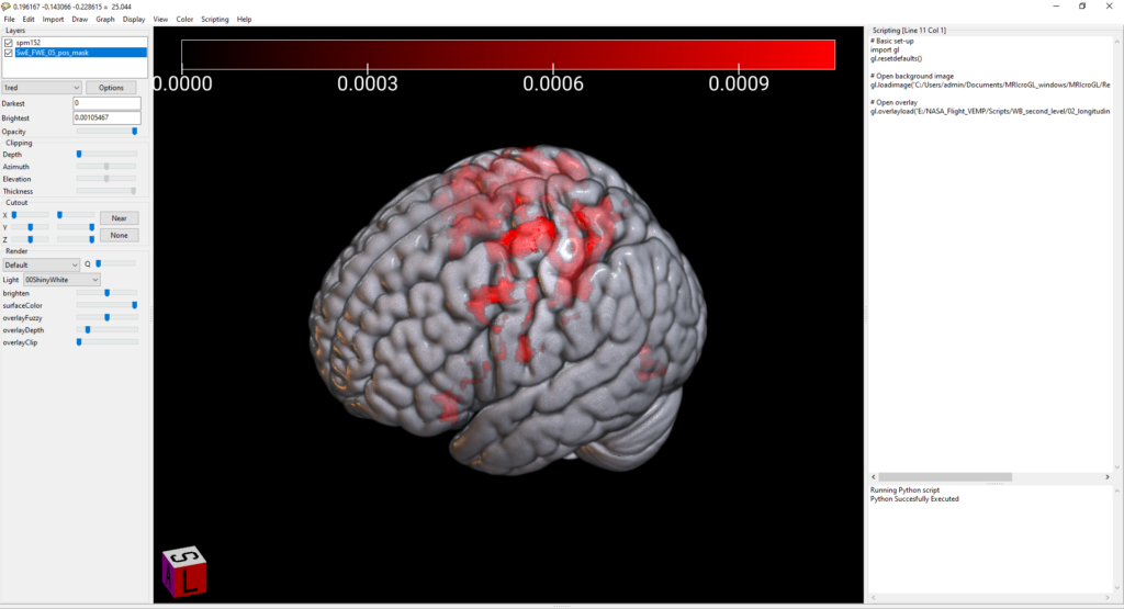
Set color options

Now you can select the color options for your overlay. I’ve selected the color called “4hot.” You can click through the different color options in the drop-down menu and then grab the name of the color you like best. I believe there’s also options for creating custom color palates, but I’ve never needed to do this so I’m not sure. The wiki page or NITRC help page likely discuss custom color options further.

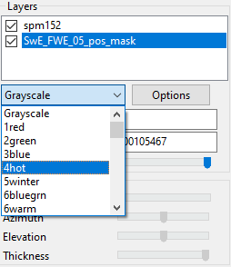
Add the color of your choice to your code. I’ve picked 4hot here. Note that you need (1, “4hot”). The 1 is referring to your first overlay. If you had >1 overlay (e.g., positive and negative results) you would use (2, “second_color”) for the second overlay, (3, “third_color”) for the third, etc. Then, set the min and max values for displaying this overlay. The numbers you need here are going to depend entirely on what type of image you’re overlaying and what the numbers in that image are. I’ve set the min (for overlay #1) to 0 and the max to 5. Note: if you need to change the min-max for the underlay (template) image, this is image 0; so you could use gl.minmax(0, 0, 100) to set the template min-max from 0-100. Lastly, I’m leaving in the opacity code here. You can use this to set the opacity of the overlay. I have opacity set to 100% here (higher = more opaque) which doesn’t do anything; however, e.g., if you had two overlays with some overlap you could use this line of code to make the opacity lower.

# Set overlay display parameters; 1 indicates 1st overlay
gl.colorname(1,"4hot")
gl.minmax(1, 0, 5)
gl.opacity(1, 100)

Now, my image is starting to look a bit nicer:

Set overlay smoothing

When you’re adding overlays you can also set whether or not you want them to be smoothed or not. Set to 1 for “smoothed interpolation” and to 0 for “jagged interpolation.”

# Put this line *before* your gl.overlayload('Filename') command
## Jagged interpolation of overlay 
gl.overlayloadsmooth(0)

## Smooth interpolation of overlay 
gl.overlayloadsmooth(1)

I didn’t worry about this for that whole brain image I’m working on because the activation cluster was very big and widespread (i.e., the orange above). However, this setting did make a difference when working with tiny cerebellar clusters. It appears that — if you don’t use this command — you get smooth interpolation (=1). For these small clusters, I was a bit surprised, I thought that smooth interpolation would make the clusters appear larger (and perhaps too large compared compared to their “actual” size); however, I found the opposite. Jagged interpolation produced bigger-looking clusters. I will dig into this a big more as to which option is most “correct” for these tiny clusters. It might be that — in the smoothed version — some of the “real” activation gets smoothed away when interpolating with areas of no activation outside of the cluster (and this is a lot more pronounced when we’re looking at small clusters in small cerebellar structures). Worth, however, considering and digging into smoothing options.

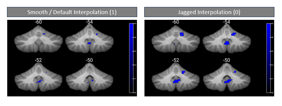
Update: when we check out how smooth vs. jagged interpolation affects nice, big clusters we do not see *much* difference between the two options (although we still see some!). In this case selecting either option won’t change your visual display much — but if you’re showing results that are already statistically thresholded, you probably want to turn smoothing off… That is, you likely want your results to appear exactly as they do in your SPM glass brain, with no visual alterations. Further, it is super important to be aware of this setting when working with small clusters. This can save you quite a headache; if you have very very tiny clusters (e.g., k=10-15), using smooth interpolation may cause them to disappear totally from your image!

Mess with the color bar

There are several (but relatively limited) options to play around with the color bar (i.e., the gradient bar that goes from your min to max overlay color values that you specified above). You can set the position to 0 = off (no color bar), 1 = top, or 2 = right. It does not look like you can set it to left or bottom, which is odd; e.g., 3 doesn’t do anything. You can also set the color bar size. You’ll have to play with this some, but for me 0.05 looks like a nice size. According to the GitHub page, this should be a value from 0.01 to 0.5 that specifies the “fraction of the screen used by the colorbar” –> aka, likely something you’ll need to play around with to get how you like, but you should be trying values from 0.01 to 0.5. Also, don’t worry here or once you’ve created the mosaic of slices if it looks like your colorbar proportions are not right compared to your image. This gets fixed later on when you save the image.

# Set color bar options 
gl.colorbarposition(2)
gl.colorbarsize(0.05)

Orient the render to your liking

I am not doing this here, but if you wanted to play more with the rendered image and use only that, you can also tweak the orientation of the rendered brain. You can run gl.viewaxial(0 or 1) to display the bottom or top of the brain, gl.viewcoronal(0 or 1) to display the front or back of the brain, or gl.viewsagittal(0 or 1) to display the right or left side of the brain. However, note that you can only run one of these commands, not all of them. Whichever command you run last is the one that will be there in your final image. What I’m not sure is whether you can script to tilt the rendered brain to an angle in between these straight-on views. This is not a goal of mine right now, so I won’t play with it further — but that may be worth asking on the help forum in the future if the GitHub page doesn’t provide an option for this.

# Set render angle to view the left side of the brain
gl.viewsagittal(1)

Select slices for mosaic

You could just stop here if you only want a rendered brain — but in my case, I want to show brain slices as well. Thus, I’ll add a line that asks for a “mosaic” of slices.

# Set mosaic slices 
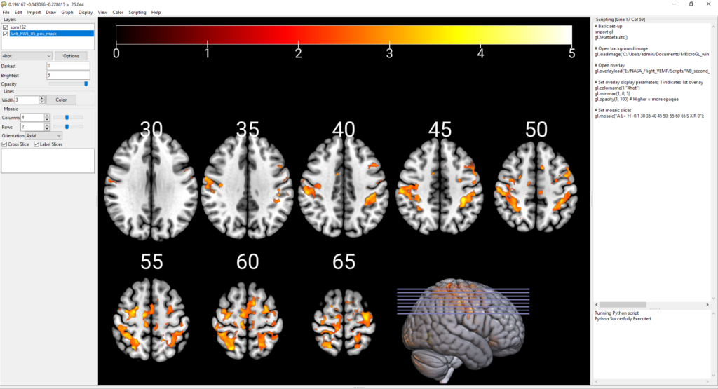
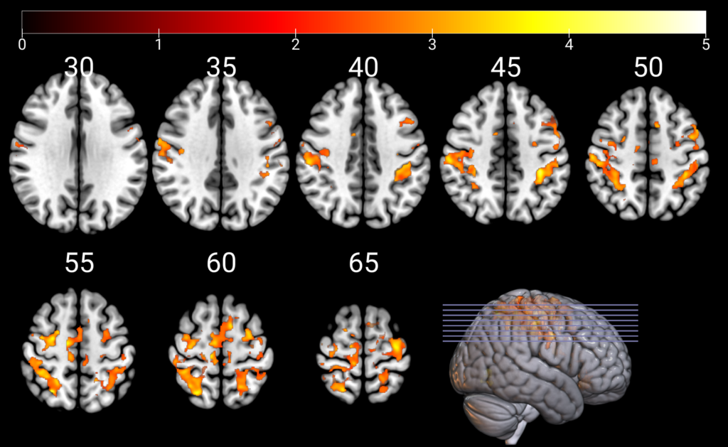
gl.mosaic("A L+ H -0.2 30 35 40 45 50; 55 60 65 S X R 0");

Let’s break down this command:

• A = axial slices (display axial slices). Other options here are C = coronal slices, or S = sagittal slices.
• L+ = labels. Display slice number labels for each slice. Other options are L- if you don’t want to display slice numbers.
• H -0.2 = horizontal overlap. This sets the horizontal overlap (or closeness) of slices. At -0.2, your slices overlap some in the horizontal direction (this is useful if you’re trying to cram a lot of slices into a small figure space and/or if you don’t have interesting results on the edges of your brain slices). If you want no horizontal overlap, set H 0 or maybe H -0.1. If you want a lot of overlap, set e.g., H -0.6. You can also set vertical overlap. Just use e.g., V -0.8 to tell your slices to vertically overlap. What’s probably more practical here is to use a smaller factor like V -0.2 to get your slices vertically closer together (e.g., to save space), but not have them overlap each other (which might look messy in the vertical direction).
• 30 35 40 45 50; 55 60 65 = the slice numbers to display. You’ll want to play with this a bit to determine the optimal slices to show for your results. E.g., there’s (probably) no sense in displaying slices with no significant results; you likely want to get a nice mix of slices that show your interesting results. Note that the semicolon separates rows. You can make a bunch of rows if you add extra semicolons. Here I have 5 slices on my top row and 3 on the bottom row (which you’ll see allows the rendered brain to fit in nicely on the bottom row).
• S X R O = sagittal rendered brain with lines to indicate reference slices. S = sagittal render. Similar to above where we chose the view for the slices, you could alternatively use A = axial rendered brain or C = coronal rendered brain. X puts reference lines through the brain at the locations of your selected slices. If you delete the X, you get rid of these purple reference lines. R = render. This asks for a rendered brain to serve as the reference; alternatively, you can delete the R and instead you’ll just get a slice as the reference. 0 = slice 0 is the reference. I really don’t think this makes a difference for a rendered brain? However, if you delete the 0, you delete the rendered brain. This is specifying which slice to use as the reference image slice. If you delete the R and instead want e.g., a single sagittal slice as the reference this does matter, because you are specifying whether you want the midsagittal slice (slice 0) versus some other slice as the reference. On a rendered brain, you seem to get an identical image (e.g., no altering of the rendered brain orientation) specifying 0 or 20, so you can likely ignore this but just keep a 0 here if you want a rendered brain.

Now, with the mosaic slice settings in place, our image is looking much nicer:

Update: to include slices from >1 plane, just add extra A / S / C commands. E.g., here, I ask for slice #38 in the axial (A) plane, slice #-25 in the sagittal (S) plane, and slice #-15 in the coronal (C) plane:

# Set mosaic slices
gl.mosaic("A L- H 0 38 S -25 C -15");

And produce this:

Check that you know which side is left vs. right

This is super important. You need to know whether you’re viewing your images in radiological view (left = right, right = left) or neurological view (left = left, right = right). It’s super useful that MRIcroGL can handle both settings (e.g., a doctor might want images in radiological, whereas neuro research folks probably want images in neurological view). Despite this, the menu selection to toggle radiological vs. neurological view is a little tricky to find. To set this in your MRIcroGL, go to: Help > Preferences > Toggle Radiological convention on vs. off.

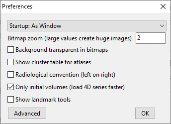
I’ve honestly never seen this menu before because it is a little hidden under the Help tab, rather than under File, View, etc. However, it is super useful. It has some other very useful options in the GUI (e.g., load only the first volume if opening a big fMRI time series). Also, if you select Advanced, you get a text file with a ton of other options — definitely worth exploring! Note, too, that it looks like when you alter these options (as expected), the next time you open MRIcroGL they will stick. So if you set to radiological view and reopen MRIcroGL it’ll stay in radiological view (& you can verify this with the Left (L) and Right (R) labels in multi-planar view).

Save the image

Now all that’s left to do is save your image in a high enough resolution that it’ll work for papers, talks, and posters. For this you can use the gl.savebmp function to save the image as a PNG to a specified path.

# Save the image 
gl.savebmp('E:/Scripts/WB_second_level/02_longitudinal_SwE/figs/SwE_FWE_05_pos.png')

& there you go! Now you’ve got a nice high-resolution image. It appears that you can use another function, bmpzoom, to save at an even higher resolution. The savebmp defaults seem to work fine for me (& e.g., are high enough resolution that you get no blurring of brain or text when zooming into the image), but this is worth noting in case you need to achieve a higher resolution image. See here for more info on bmpzoom.

Update: Note that in the above Help > Preferences window, you can also set the bmpzoom manually. E.g., I’ve found that ~2 is too small to get nice, not-blurry images for pubs. Higher numbers, such as ~4-8 make the text (e.g., the slice and colorbar numbers) look a lot better.

All of the mosaic code

For reference, here’s the mosaic code all in one place. As described above, I saved this code as a *.py file so that I can reopen it to recreate this image easily, and so that I can tweak it whenever I need to create other similar images.

# Basic set-up 
import gl
gl.resetdefaults()

# Open background image
gl.loadimage('C:/Users/admin/Documents/MRIcroGL_windows/MRIcroGL/Resources/standard/spm152.nii')

# Jagged (0) or smooth (1) interpolation of overlay  
gl.overlayloadsmooth(0)

# Open overlay
gl.overlayload('E:/Scripts/WB_second_level/02_longitudinal_SwE/set1_BG_masked/SwE_FWE_05_pos_mask.nii')

# Set overlay display parameters; 1 indicates 1st overlay
gl.colorname(1,"4hot")
gl.minmax(1, 0, 5)
gl.opacity(1, 100)

# Set the color bar options 
gl.colorbarposition(2)
gl.colorbarsize(0.05)

# Set mosaic slices 
gl.mosaic("A L+ H -0.1 30 35 40 45 50; 55 60 65 S X R 0");

# Save the image 
gl.savebmp('E:/Scripts/WB_second_level/02_longitudinal_SwE/figs/SwE_FWE_05_pos.png')

Updates

Changing the render style:
Sometimes the default render setting is too “shiny.” It makes it tricky to see if you have very bright activation spots. One solution to this is to change your render style from default to e.g., matte.

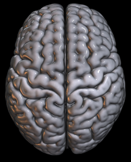
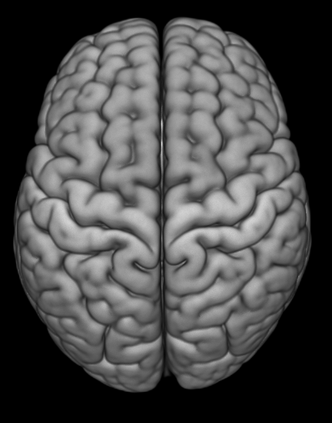
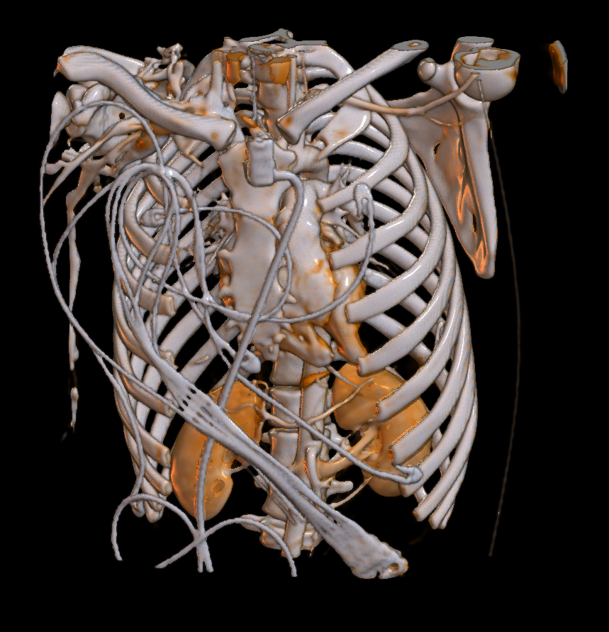
Here’s the line of code to add in. You change the shadername property. Depending on your goals, you can play with the shader options to get some interesting effects; for instance, there’s a glass brain option to make the brain transparent — which is perhaps not useful for a final manuscript figure, but maybe is useful for depicting study statistical results to share with your coauthors.

gl.shadername('matte')

Playing with the render cutout:
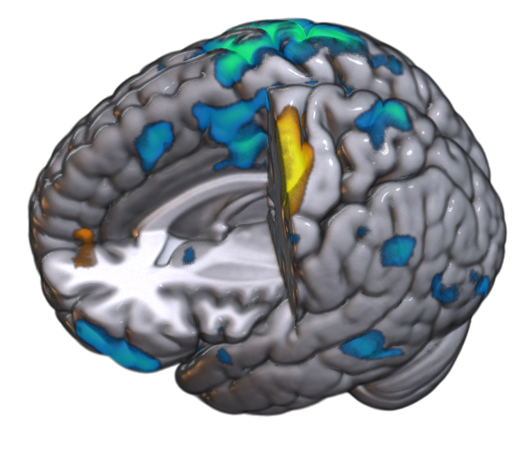
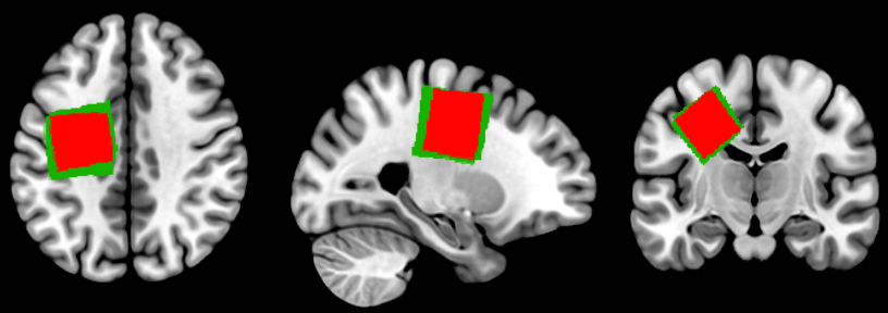
This is still tripping me up some, but a hugely useful feature of MRIcroGL is the ability to do cut outs, i.e., to chop out part of the brain to show internal results on a 3D rendered brain. First off, you want to consider whether to show the overlay in the area that’s being cut out. You may *not* want to do this if you want to show floating results, like some fMRI results blobs floating in a cut out space. However, in this specific case, I was showing age difference results, so I had a *ton* of young > old results. I wanted to make some cutouts to show e.g., mid-sagittal slices. If I let my results overlay stay in the regions I cut out, this didn’t help me at all:

However, if I set the overlay to be ‘hidden’ by the cutout, this fixes my problem:

#first 1 indicates overlay #1
#second 1 indicates YES, hide my overlay by my cutout
gl.hiddenbycutout(1,1)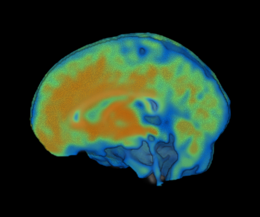

I’m still figuring exactly how to work with the cutout function. So, for now, here is the cutout function documentation and just a couple of examples to hopefully get you started:

# Cutout function documentation: gl.cutout(L,A,S,R,P,I)

# To get the left hemisphere only: 
gl.cutout(1,1,1,0.5,0,0)

# To get the right hemisphere only: 
gl.cutout(0.5,0,1,0,1,0)

All of the commands!

Another new thing I just found: if you go to Scripting > Templates > help, you can print a long list of example functions. I’ve copied this below. Make sure, however, that you put ‘gl.’ in front of any of these functions before running your python script! Also this help documentation notes a way to print all functions, which could be super helpful!

The gl module displays NIfTI format images
 To see all functions: "print(dir(gl))"
 To see details for a specific function: "print(gl.wait.__doc__)"

azimuthelevation (built-in function): 
 azimuthelevation(azi, elev) -> Sets the camera location.
backcolor (built-in function): 
 backcolor(r, g, b) -> changes the background color, for example backcolor(255, 0, 0) will set a bright red background
bmpzoom (built-in function): 
 bmpzoom(z) -> changes resolution of savebmp(), for example bmpzoom(2) will save bitmaps at twice screen resolution
cameradistance (built-in function): 
 cameradistance(z) -> Sets the viewing distance from the object.
clipazimuthelevation (built-in function): 
 clipazimuthelevation(depth, azi, elev) -> Set a view-point independent clip plane.
clipthick (built-in function): 
 clipthick(thick) -> Set size of clip plane slab (0..1).
colorbarposition (built-in function): 
 colorbarposition(p) -> Set colorbar position (0=off, 1=top, 2=right).
colorbarsize (built-in function): 
 colorbarsize(p) -> Change width of color bar f is a value 0.01..0.5 that specifies the fraction of the screen used by the colorbar.
coloreditor (built-in function): 
 coloreditor(s) -> Show (1) or hide (0) color editor and histogram.
colorfromzero (built-in function): 
 colorfromzero(layer, isFromZero) -> Color scheme display range from zero (1) or from treshold value (0)?
colorname (built-in function): 
 colorname(layer, colorName) -> Set the colorscheme for the target overlay (0=background layer) to a specified name.
cutout (built-in function): 
 cutout(L,A,S,R,P,I) -> Remove sector from volume.
extract (built-in function): 
 extract(|b,s,t) -> Remove haze from background image. Blur edges (b: 0=no, 1=yes, default), single object (s: 0=no, 1=yes, default), threshold (t: 1..5=high threshold, 5 is default, higher values yield larger objects)
fullscreen (built-in function): 
 fullscreen(max) -> Form expands to size of screen (1) or size is maximized (0).
generateclusters (built-in function): 
 generateclusters(layer |,thresh, minClusterMM3, method, bimodal) -> create list of distinct regions. Optionally provide cluster intensity, minimum cluster size, neighbor method(1=faces,2=faces+edges,3=faces+edges+corners). If bimodal = 1, both dark and bri
ght clusters are detected.
graphscaling (built-in function): 
 graphscaling(type) -> Vertical axis of graph is raw (0), demeaned (1) normalized -1..1 (2) normalized 0..1 (3) or percent (4).
hiddenbycutout (built-in function): 
 hiddenbycutout(layer, isHidden) -> Will cutout hide (1) or show (0) this layer?
invertcolor (built-in function): 
 invertcolor(layer, isInverted) -> Is color intensity inverted (1) or not (0) this layer?
linecolor (built-in function): 
 linecolor(r,g,b) -> Set color of crosshairs, so "linecolor(255,0,0)" will use bright red lines.
linewidth (built-in function): 
 linewidth(wid) -> Set thickness of crosshairs used on 2D slices.
loadgraph (built-in function): 
 loadgraph(graphName, add = 0) -> Load text file graph (e.g. AFNI .1D, FSL .par, SPM rp_.txt). If "add" equals 1 new graph added to existing graph
loadimage (built-in function): 
 loadimage(imageName) -> Close all open images and load new background image.
minmax (built-in function): 
 minmax(layer, min, max) -> Sets the color range for the overlay (layer 0 = background).
modalmessage (built-in function): 
 modalmessage(msg) -> Show a message in a dialog box, pause script until user presses "OK" button.
mosaic (built-in function): 
 mosaic(mosString) -> Create a series of 2D slices.
opacity (built-in function): 
 opacity(layer, opacityPct) -> Make the layer (0 for background, 1 for 1st overlay) transparent(0), translucent (~50) or opaque (100).
orthoviewmm (built-in function): 
 orthoviewmm(x,y,z) -> Show 3 orthogonal slices of the brain, specified in millimeters.
overlayadditiveblending (built-in function): 
 overlayadditiveblending(v) -> Merge overlays using additive (1) or multiplicative (0) blending.
overlaycloseall (built-in function): 
 overlaycloseall() -> Close all open overlays.
overlayload (built-in function): 
 overlayload(filename) -> Load an image on top of prior images.
overlayloadsmooth (built-in function): 
 overlayloadsmooth(0) -> Will future overlayload() calls use smooth (1) or jagged (0) interpolation?
overlaymaskwithbackground (built-in function): 
overlaymaskwithbackground(v) -> hide (1) or show (0) overlay voxels that are transparent in background image.
quit (built-in function): 
 quit() -> Terminate the application.
removesmallclusters (built-in function): 
 removesmallclusters(layer, thresh, mm, neighbors) -> only keep clusters where intensity exceeds thresh and size exceed mm. Clusters based on neighbors that share faces (1), faces+edges (2) or faces+edges+corners (3)
resetdefaults (built-in function): 
 resetdefaults() -> Revert settings to sensible values.
savebmp (built-in function): 
 savebmp(pngName) -> Save screen display as bitmap. For example "savebmp('test.png')"
scriptformvisible (built-in function): 
 scriptformvisible (visible) -> Show (1) or hide (0) the scripting window.
shaderadjust (built-in function): 
 shaderadjust(sliderName, sliderValue) -> Set level of shader property. Example "gl.shaderadjust('edgethresh', 0.6)"
shaderlightazimuthelevation (built-in function): 
 shaderlightazimuthelevation(a,e) -> Position the light that illuminates the rendering. For example, "shaderlightazimuthelevation(0,45)" places a light 45-degrees above the object
shadermatcap (built-in function): 
 shadermatcap(name) -> Set material capture file (assumes "matcap" shader. For example, "shadermatcap('mc01')" selects mc01 matcap.
shadername (built-in function): 
 shadername(name) -> Choose rendering shader function. For example, "shadername('mip')" renders a maximum intensity projection.
shaderquality1to10 (built-in function): 
 shaderquality1to10(i) -> Renderings can be fast (1) or high quality (10), medium values (6) balance speed and quality.
shaderupdategradients (built-in function): 
 shaderupdategradients() -> Recalculate volume properties.
sharpen (built-in function): 
 sharpen() -> apply unsharp mask to background volume to enhance edges
smooth (built-in function): 
 smooth2D(s) -> make 2D images blurry (linear interpolation, 1) or jagged (nearest neightbor, 0).
toolformvisible (built-in function): 
 toolformvisible(visible) -> Show (1) or hide (0) the tool panel.
version (built-in function): 
 version() -> Return the version of MRIcroGL.
view (built-in function): 
 view(v) -> Display Axial (1), Coronal (2), Sagittal (4), Flipped Sagittal (8), MPR (16), Mosaic (32) or Rendering (64)
viewaxial (built-in function): 
 viewaxial(SI) -> Show rendering with camera superior (1) or inferior (0) of volume.
viewcoronal (built-in function): 
 viewcoronal(AP) -> Show rendering with camera posterior (1) or anterior (0) of volume.
viewsagittal (built-in function): 
 viewsagittal(LR) -> Show rendering with camera left (1) or right (0) of volume.
volume (built-in function): 
 volume(layer, vol) -> For 4D images, set displayed volume (layer 0 = background; volume 0 = first volume in layer).
wait (built-in function): 
 wait(ms) -> Pause script for (at least) the desired milliseconds.
zerointensityinvisible (built-in function): 
 zerointensityinvisible(layer, bool) ->  For specified layer (0 = background) should voxels with intensity 0 be opaque (bool= 0) or transparent (bool = 1).
zoomcenter (built-in function): 
 zoomcenter(x,y,z) -> Set center of expansion for zoom scale (values in range 0..1 with 0.5 in volume center).
zoomscale (built-in function): 
 zoomscale2D(z) -> Enlarge 2D image (range 1..6).