Here I’m going to create a running list of random tips for the ggplot2 library in R.
Setting up axes
Pull the X and Y axis limits to view or use them when you’ve let ggplot automatically set the axes:
# Pull x axis limits for plot named g1
ggplot_build(g1)$layout$panel_scales_x[[1]]$range$range

# Pull y axis limits for plot named g1
ggplot_build(g1)$layout$panel_scales_y[[1]]$range$range

# An alternative way to do the same as above
layer_scales(g1)$x$range$range; layer_scales(g1)$y$range$range
Set the X and Y axes to pre-defined limits; this is the most basic way to alter the x and y axis limits, but often does the job just fine.
+ xlim=c(0,20) + ylim=c(0,150)Define the specific breaks you want in an axis; this specifies breaks at -1, -0.5, 0, and 0.3. This is for a small graph where I only want these four labels on the y axis.
+ scale_y_continuous(breaks=c(-1,-0.5,0,0.3))Adding shapes and text
Add a rectangle to your plot, e.g., to show the duration of an intervention on a longitudinal plot.
# Code to add a blue rectangle to your plot
+ geom_rect(mapping=aes(xmin=0, xmax=188.13, ymin=-0.8, ymax=0.17), fill="dodgerblue", alpha=0.03, linetype=0)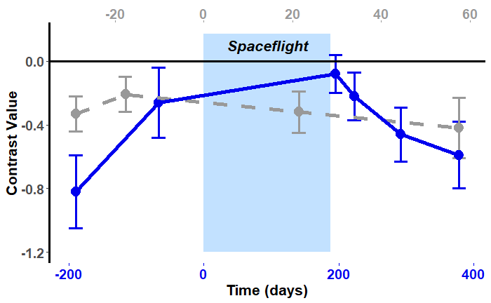
Add text to your plot, e.g., to label your rectangle.
# Add text at a certain spot on your plot
+ annotate("text", x=95, y=0.10, label="Spaceflight", size=5.5, fontface="bold.italic")
Add subject number labels to your plot to label which point corresponds to each subject, e.g., to identify outlier subject numbers.
+ geom_text(aes(label=Subj))Tweaking colors
Make the background of a plot all black, instead of default (white). See this site for more information and options. This was the only code I needed to add to my correlation plot code to make a black background:
# Code to add for black background
+ theme(panel.background=element_rect(fill="black"),
      plot.background=element_rect(fill="black"))
Here’s the full code for this plot, for reference:
# Full code for this plot
g1 <- ggplot(data_Flight01, aes(x=SOT_post_pre, y=SOT_beta_38_neg14_46_change)) +
     geom_point(size=5.5,color="blue2") + theme_classic() +
     labs(x="SOT Score Change",y="Contrast Value Change") +
     theme(plot.title=element_text(size=22, face="bold", hjust = 0.5)) +
     theme(axis.title=element_text(size=20, face="bold", color="white"),
              axis.text=element_text(size=15, face="bold", color="white")) +
     geom_hline(yintercept=0, linetype="dashed", color="white", size=1) +
     theme(panel.background=element_rect(fill="black"),
           plot.background=element_rect(fill="black"))
g1
Before:
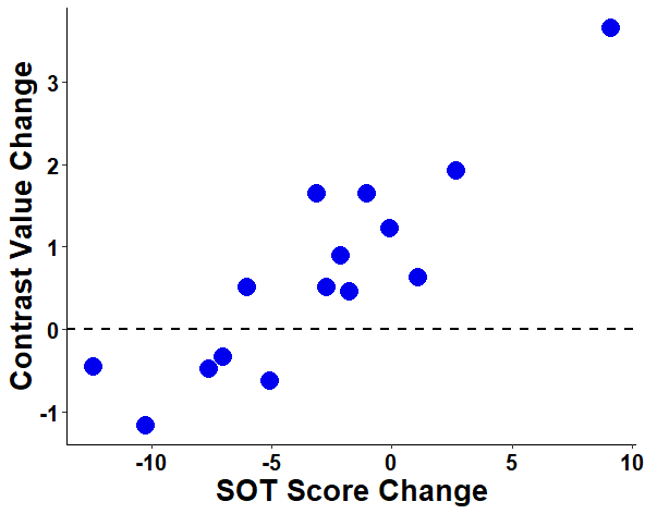
After:

Change the transparency of a geom_point; e.g., if you have some overlapping points this could help.
# Set the alpha to indicate your desired amount of transparency
+ geom_point(size=5.5,color="blue2",alpha=0.5)*For cheat-sheet lists of colors available in R, see:
http://www.stat.columbia.edu/~tzheng/files/Rcolor.pdf
Making a boxplot for two groups
Here’s some starter code for making two side-by-side boxplots to show a variable for two different groups. Note that I used geom_jitter to squiggle the points around laterally a little, instead of having them all stacked directly up in a straight line. You could use geom_point instead if that’s what you wanted (or, you could set the width and height of the jitter both to 0).
# Boxplot of group difs
g1 <- ggplot(dataFrontalVoxelGSH, aes(x=Age_Group, y=Frontal_GSH_ConcIU_TissCorr)) +
      geom_boxplot(aes(color=Age_Group),lwd=1.2) +

      scale_color_manual(values=c('darkorange2','dodgerblue')) +
      theme_classic() +
      theme(legend.position="none") +
      labs(y="Tissue-Corrected GSH", x="Age Group") +
      theme(axis.title=element_text(size=20, face="bold"), axis.text=element_text(size=16, face="bold")) +
      geom_jitter(width = 0.05, height = 0, size = 3.5, aes(color=Age_Group)) +
      scale_shape_manual(values=c(19))
g1
ggsave(g1, file = "G:/Shared drives/GABA_Aging_GSH/Manuscript_Figures/TissCorr_Frontal_GSH.png", dpi = 400)
Here’s what the plot from the above code looks like:

Revamping your boxplots into raincloud plots
I’ve been told that raincloud plots are the new boxplots. Raincloud isn’t built into ggplot2 (yet), so you have to do a little set-up first. For this, I’ve used code from David Robinson’s GitHub page.
So, I have a little R code snippet that sets up the violin plot function. Again, not mine, but from this helpful GitHub page.
```{r Set up violin plot funct}

# Function for making violin plot
#   https://gist.github.com/dgrtwo/eb7750e74997891d7c20
# somewhat hackish solution to:
# https://twitter.com/EamonCaddigan/status/646759751242620928
# based mostly on copy/pasting from ggplot2 geom_violin source:
# https://github.com/hadley/ggplot2/blob/master/R/geom-violin.r

library(ggplot2)
library(dplyr)


"%||%" <- function(a, b) {
  if (!is.null(a)) a else b
}

geom_flat_violin <- function(mapping = NULL, data = NULL, stat = "ydensity",
                        position = "dodge", trim = TRUE, scale = "area",
                        show.legend = NA, inherit.aes = TRUE, ...) {
  layer(
    data = data,
    mapping = mapping,
    stat = stat,
    geom = GeomFlatViolin,
    position = position,
    show.legend = show.legend,
    inherit.aes = inherit.aes,
    params = list(
      trim = trim,
      scale = scale,
      ...
    )
  )
}

#' @rdname ggplot2-ggproto
#' @format NULL
#' @usage NULL
#' @export
GeomFlatViolin <-
  ggproto("GeomFlatViolin", Geom,
          setup_data = function(data, params) {
            data$width <- data$width %||%
              params$width %||% (resolution(data$x, FALSE) * 0.9)

            # ymin, ymax, xmin, and xmax define the bounding rectangle for each group
            data %>%
              group_by(group) %>%
              mutate(ymin = min(y),
                     ymax = max(y),
                     xmin = x,
                     xmax = x + width / 2)
          },

          draw_group = function(data, panel_scales, coord) {
            # Find the points for the line to go all the way around
            data <- transform(data, xminv = x,
                              xmaxv = x + violinwidth * (xmax - x))

            # Make sure it's sorted properly to draw the outline
            newdata <- rbind(plyr::arrange(transform(data, x = xminv), y),
                             plyr::arrange(transform(data, x = xmaxv), -y))

            # Close the polygon: set first and last point the same
            # Needed for coord_polar and such
            newdata <- rbind(newdata, newdata[1,])

            ggplot2:::ggname("geom_flat_violin", GeomPolygon$draw_panel(newdata, panel_scales, coord))
          },

          draw_key = draw_key_polygon,

          default_aes = aes(weight = 1, colour = "grey20", fill = "white", size = 0.5,
                            alpha = NA, linetype = "solid"),

          required_aes = c("x", "y")
)

```
After I run this code to set up violin plots, I can make as many raincloud plots as I’d like, using code like this–combining violin plot with boxplot, all in a ggplot:
g1 <- ggplot(dataFrontalVoxelGSH, aes(x=Age_Group, y=Frontal_GSH_ConcIU_TissCorr, fill=Age_Group, colour=Age_Group)) +
      geom_flat_violin(position=position_nudge(x=0.25, y=0), adjust=0.5, trim=TRUE, alpha=0.65, lwd=0.8) +
      geom_point(aes(color=Age_Group), position=position_jitter(width=.15), size=2) +
      geom_boxplot(aes(x=as.numeric(Age_Group)+0.04, y=Frontal_GSH_ConcIU_TissCorr), outlier.shape=NA,
                   alpha=0.3, width=0.1, lwd=0.8) +
      scale_color_manual(values=c('darkorange2','dodgerblue')) +
      scale_fill_manual(values=c('darkorange2','dodgerblue')) +
      theme_classic() +
      coord_flip() +
      guides(fill=FALSE, colour=FALSE) +
      labs(y="Tissue-Corrected GSH", x="Age Group") +
      theme(axis.title=element_text(size=15, face="bold"), axis.text=element_text(size=12, face="bold")) +
      theme(axis.ticks.y=element_blank())
ggsave(g1, file = "G:/Shared drives/GABA_Aging_GSH/Manuscript_Figures/TissCorr_Frontal_GSH_rain_noGroupLabs.png", dpi = 400) 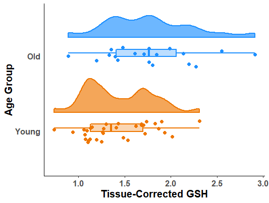
Saving ggplots
Save a high-res version of the plot and tweak other options like size, e.g., for publication-quality figures:
ggsave(g1, file = "E:/Scripts/03_behav_corr_figs/SOT_38_neg14_46.png", dpi=400, width=6.5, height=5, units="in")